Explore the Example Project

If you opted in to adding the example project during sidetrek init, you should have a fully functional data pipeline already set up.

This stack consists of the following tools:

• Dagster for orchestration
• Meltano for data ingestion
• DBT for data transformation
• Minio (local replacement for S3) and Apache Iceberg for data storage
• Trino for data querying
• Superset for data visualization

All these tools are pre-configured for you in the example project. But the data pipeline still needs to be run in order for the example data to flow through the pipeline so you can visualize them.

In this guide, we’ll walk you through how to run the example data pipeline and visualize the data in Superset.

Note that we’re going to fly through these steps - if you’re not familiar with all the tools in our stack, we strongly recommend checking out our in-depth BI Stack Example Tutorial.

TLDR; Summary of the Required Steps

• Step 1: Run the Meltano ingestion job in Dagster to load the example data into Iceberg tables.
• Step 2: Run the DBT transformations in Dagster.
• Step 3: Add Trino as a database connection in Superset and add an example dashboard.

Some Context

Before we go through these steps to run the example project, let’s quickly look at our data pipeline architecture and example dataset.

Data Pipeline Architecture

The data pipeline consists of five components:

1. Data Ingestion: First, we extract the data from our source systems (in our example, that’s the example CSV files) and load them into our storage (Minio + Iceberg) using Meltano.
2. Data Storage: This is where all the data is stored. We’re using Minio as a local replacement for S3 and Iceberg as the table format on top of Minio.
3. Data Transformation: Once the raw data is in our storage, we transform them into analytics-ready tables using DBT and Trino.
4. Orchestration: All the above steps are orchestrated by our orchestrator, Dagster.
5. Data Visualization: Finally we visualize our data in Superset.

To sum up:

Data sources (e.g. CSV files) -> Ingestion (Meltano) -> Storage (Minio + Iceberg) -> Transformation (DBT + Trino) -> Visualization (Superset)

…all orchestrated by Dagster.

The Dataset

We’ve included a simple dataset with four tables: orders (100k rows), customers (20k rows), products (2k rows), and stores (200 rows). This emulates the typical e-commerce data.

Each table has its own csv file in the /your_project/data directory.

Step 1: Data Ingestion

OK, let’s run the ingestion process to load the example data into our storage (i.e. Iceberg tables).

Data ingestion is handled by Meltano. Meltano is a managed connector with hundreds of pre-built connectors to popular data sources and targets. Essentially, it handles the EL (“Extract, Load”) part of the ELT process.

As a quick reminder, here’s where Meltano is in the project structure:

your_project
├── .sidetrek
├── .venv
├── superset
├── trino
└── your_project
    ├── dagster
    ├── data
    ├── dbt
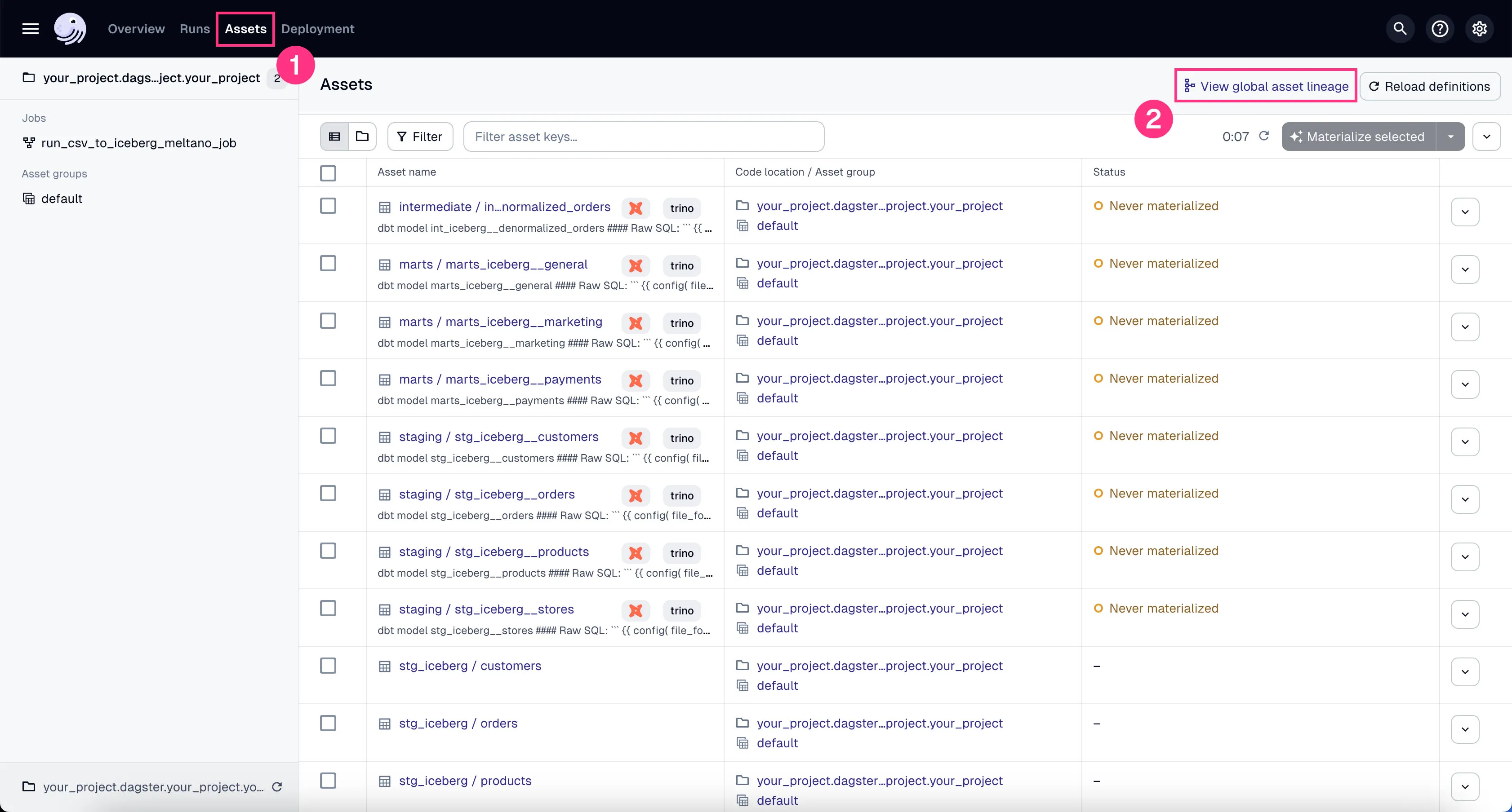
    └── meltano

We can run the Meltano ingestion job inside Dagster. In your example project, this is already set up for you.

1. Go to the Dagster dashboard at http://localhost:3000 and click on the run_csv_to_iceberg_meltano_job job

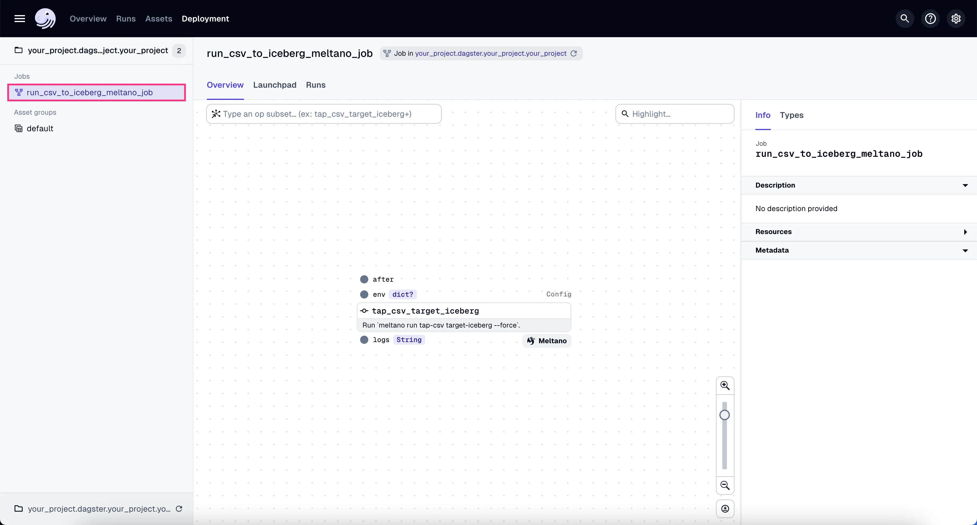
2. Go to the tab “Launchpad” and click “Launch Run”.

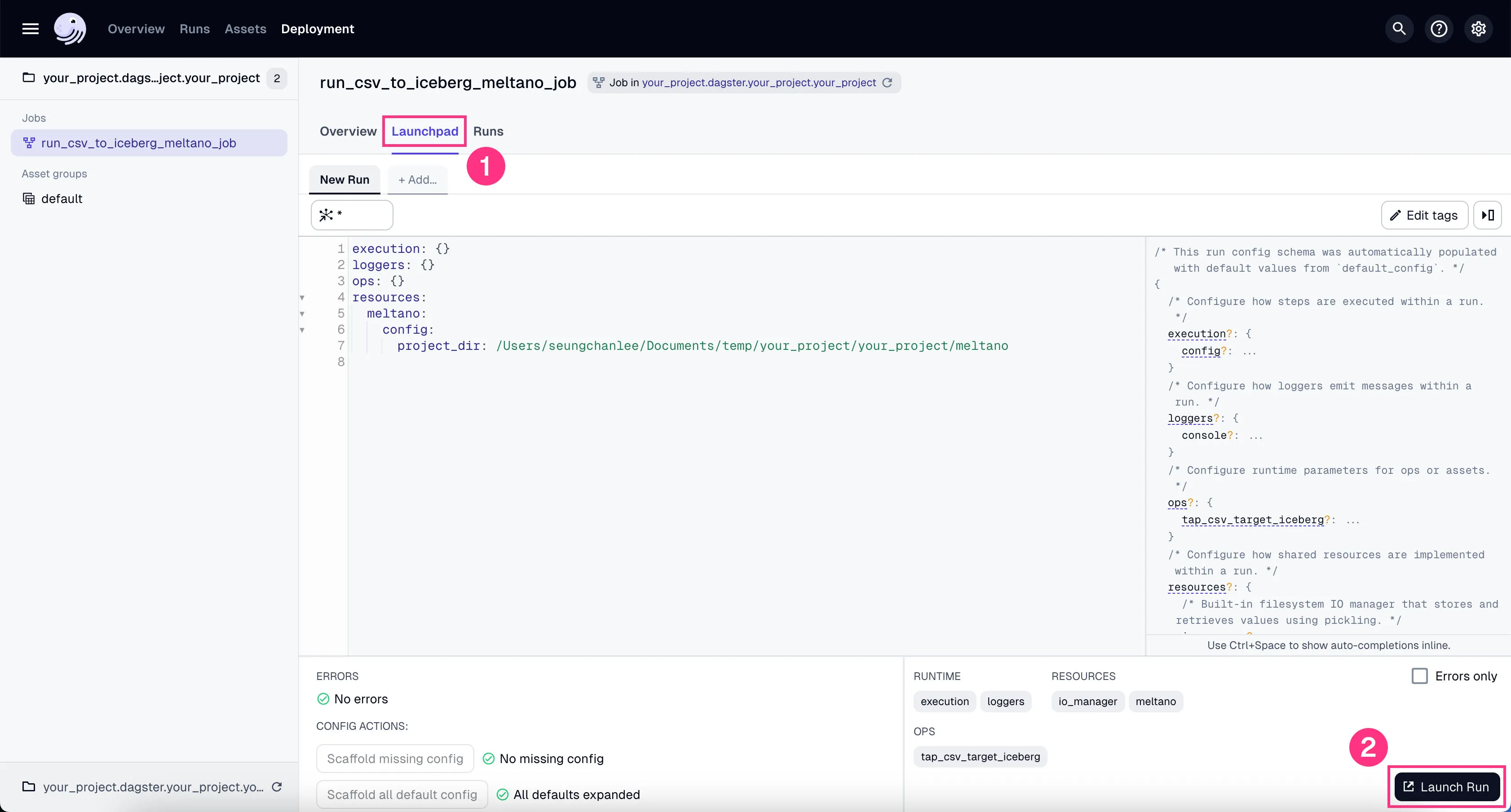
You’ll see the job starts running. It might take a couple of minutes to finish the ~100k+ rows of data we’re using in our example project.

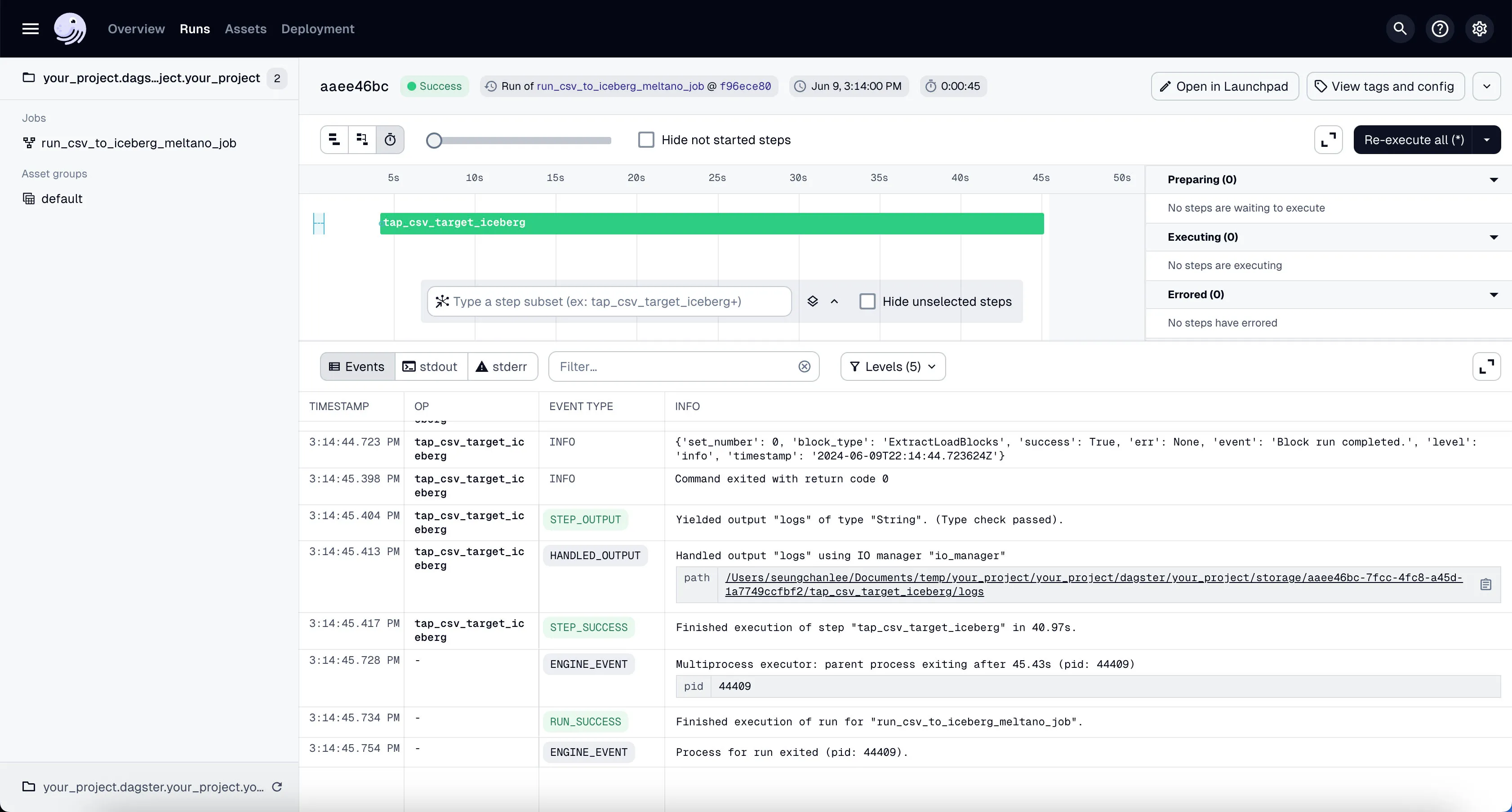
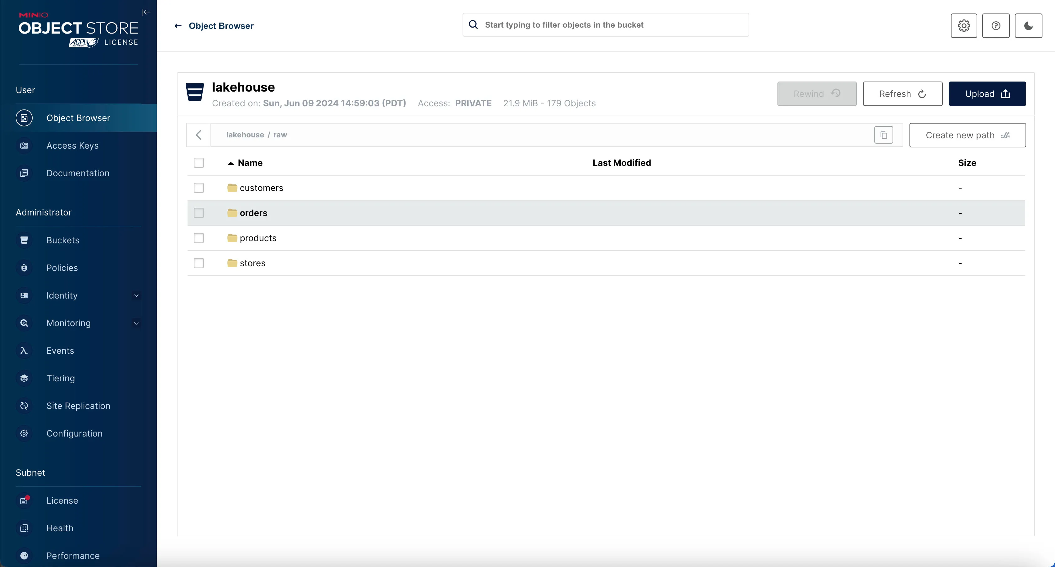
If the job is run successfully, you’ll see the 4 different tables written inside Minio’s raw directory (i.e. prefix).

Check it out in Minio by going to http://localhost:9000 and logging in with the username admin and password admin_secret.

Inspect the Iceberg Tables with Trino

We can see that there’s data in Minio, but we can’t actually query the data directly from Minio. How many rows are in each table? What data is in there?

This is where Trino comes in - we can actually query our Iceberg tables and inspect them using our query engine, Trino.

To do that, let’s enter the Trino shell.

Once you’re in the Trino shell, first you need to switch to the iceberg catalog and raw schema. This basically tells Trino we’re using the raw schema inside the Iceberg data store.

Then list out the tables in that schema.

     Table     
---------------
 orders    
 customers 
 products
 stores  
(4 rows)

To view the data inside the table, you can run something like:

This will show you the number of rows in the orders table.

  _col0  
--------
 100000 
(1 row)

Looks like our data made it in just fine!

Step 2: Data Transformation

Now that we have the data in the Iceberg tables, we can run transformation on them to turn them into analytics-ready tables.

For this, we use DBT for writing SQL for data transformation and Trino for actually executing the SQL queries DBT generates.

Trino, in turn, is connected to Iceberg where the data is actually stored so we can query them.

Finally, we connect DBT to Dagster so we can automate the running of the transformations.

In the example project, all these connections are already set up for you.

Here’s a quick reminder of where dbt and Trino are in the project structure.

your_project
├── .sidetrek
├── .venv
├── superset
├── trino
└── your_project
    ├── dagster
    ├── data
    ├── dbt
    └── meltano

Before we actually run the transformations, note that our DBT “models” (i.e. tables) are organized in three stages: staging, intermediate, and marts.

• Staging: This is where we create atomic tables from the raw data. You can think of each of these tables as the most basic unit of data — an atomic building block we’ll later compose together to build more complex SQL queries. This makes our SQL code more modular.
• Intermediate: This is where we compose a bunch of atomic tables from the staging stage to create more complex tables. You can think of this stage as an intermediate step between the modular tables in the staging stage and the final, business-conformed tables in the marts stage.
• Marts: This is where you have the final, business-conformed data ready for analytics. Each mart is typically designed to be consumed by a specific function in the business, such as the finance team, marketing team, etc.

All these DBT models are imported into Dagster so we can automate them (schedule them, for example). When we import DBT models in Dagster, they are imported as Dagster “assets”.

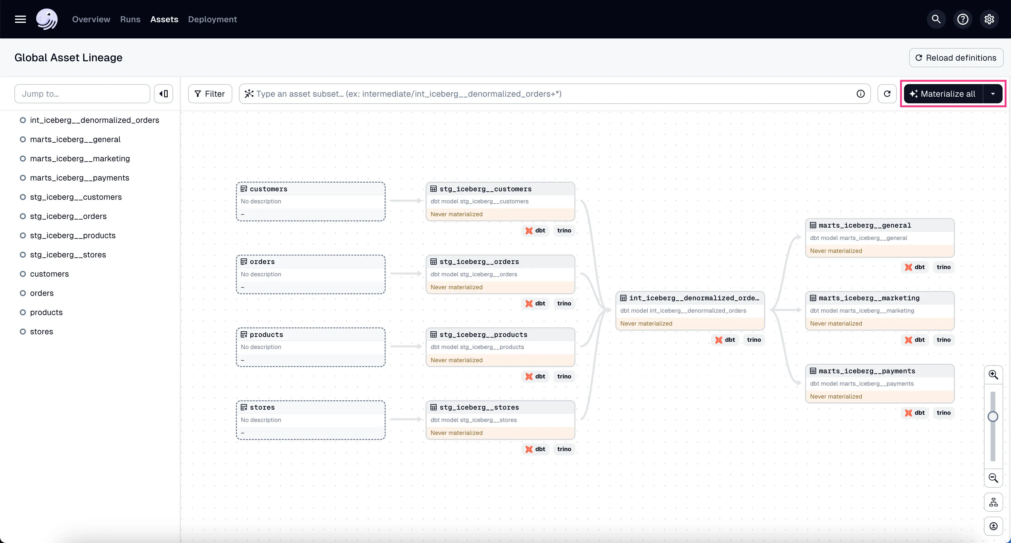
You can see all the DBT assets in Global Asset Lineage section of the Dagster dashboard:

1. Click on the “Assets” in the top menu.
2. Click on “View global asset lineage” at the top right.

In the global asset lineage view, click “Materialize all” to execute the DBT transformations (underneath, Trino is executing these DBT queries). Of course, in a production environment, you might want to schedule them instead of manually triggering them as we’re doing now.

If the materialization was successful, you should see 3 analytics-ready tables in project_marts directory (i.e. prefix) in minio.

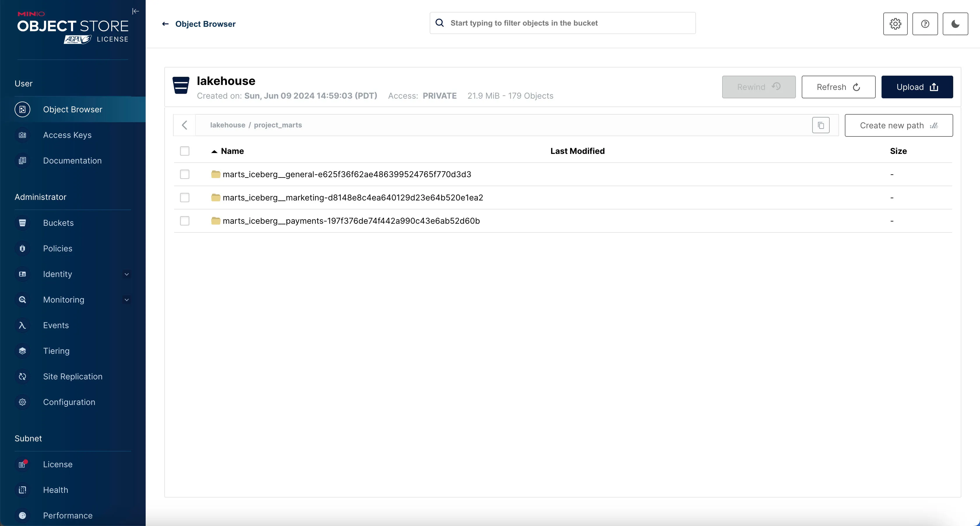
Voila! The data is now transformed and ready for analytics.

Step 3: Data Visualization

OK, now we’re ready to visualize our data. For that, we’ll use Superset.

We know that Data Analysts are particular about which tool they use here. So we’ve separated out Superset in its own directory so it can be easily replaced by another tool of your choice.

your_project
├── .sidetrek
├── .venv
├── superset
├── trino
└── your_project
    ├── dagster
    ├── data
    ├── dbt
    └── meltano

Let’s configure Superset to connect to Trino so we can visualize the data.

Superset + Trino

Go to the Superset dashboard at http://localhost:8088 and log in with the username admin and password admin.

If you’d like, you can change the username and password in the docker-init.sh file inside the superset/docker directory:

...
ADMIN_PASSWORD="admin"
...
# Create an admin user
echo_step "2" "Starting" "Setting up admin user ( admin / $ADMIN_PASSWORD )"
superset fab create-admin \
              --username admin \
              --firstname Superset \
              --lastname Admin \
              --email admin@superset.com \
              --password $ADMIN_PASSWORD

Add Trino as a Database Connection in Superset

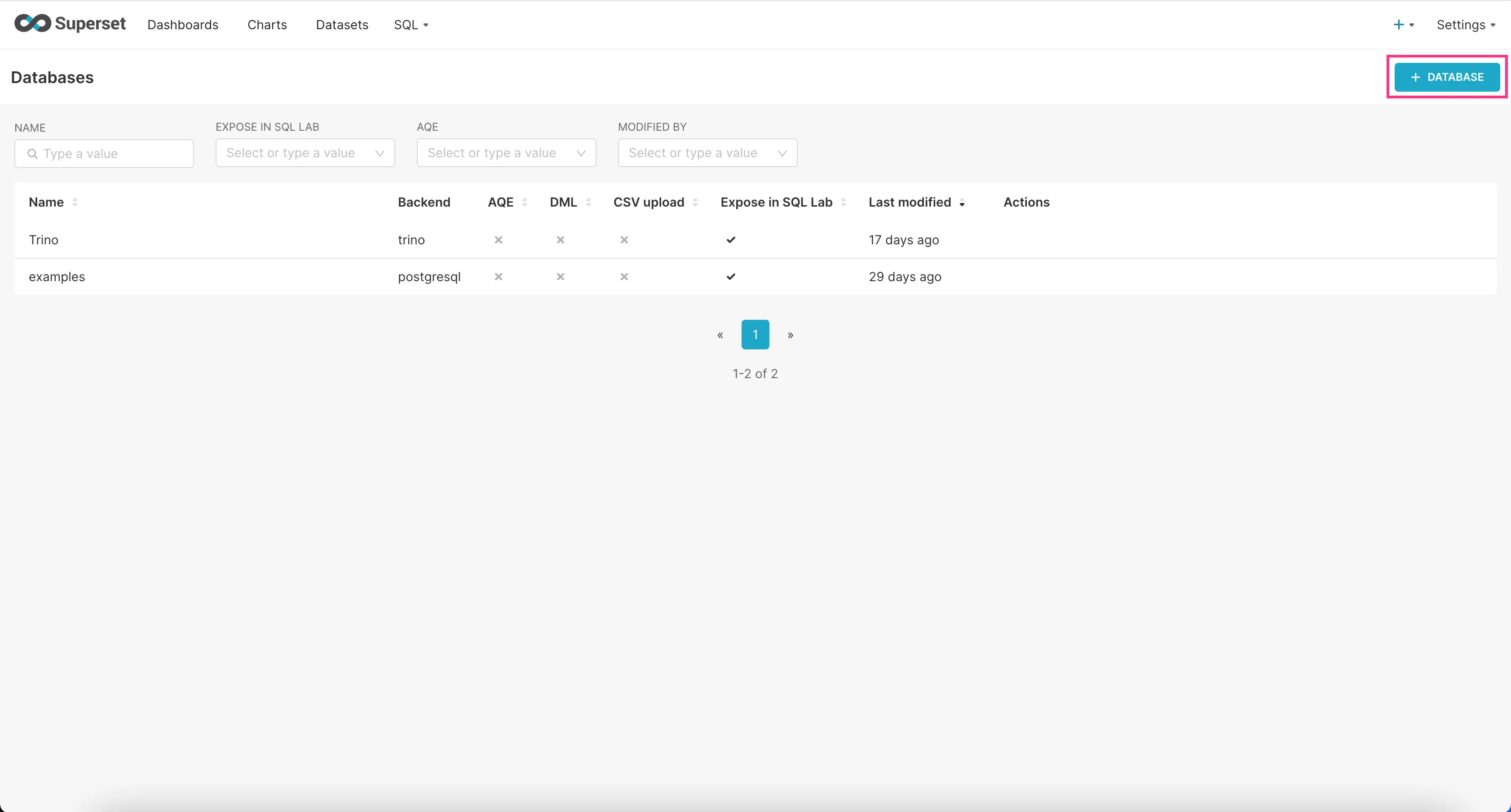
Now we need to add Trino as a database connection in Superset.

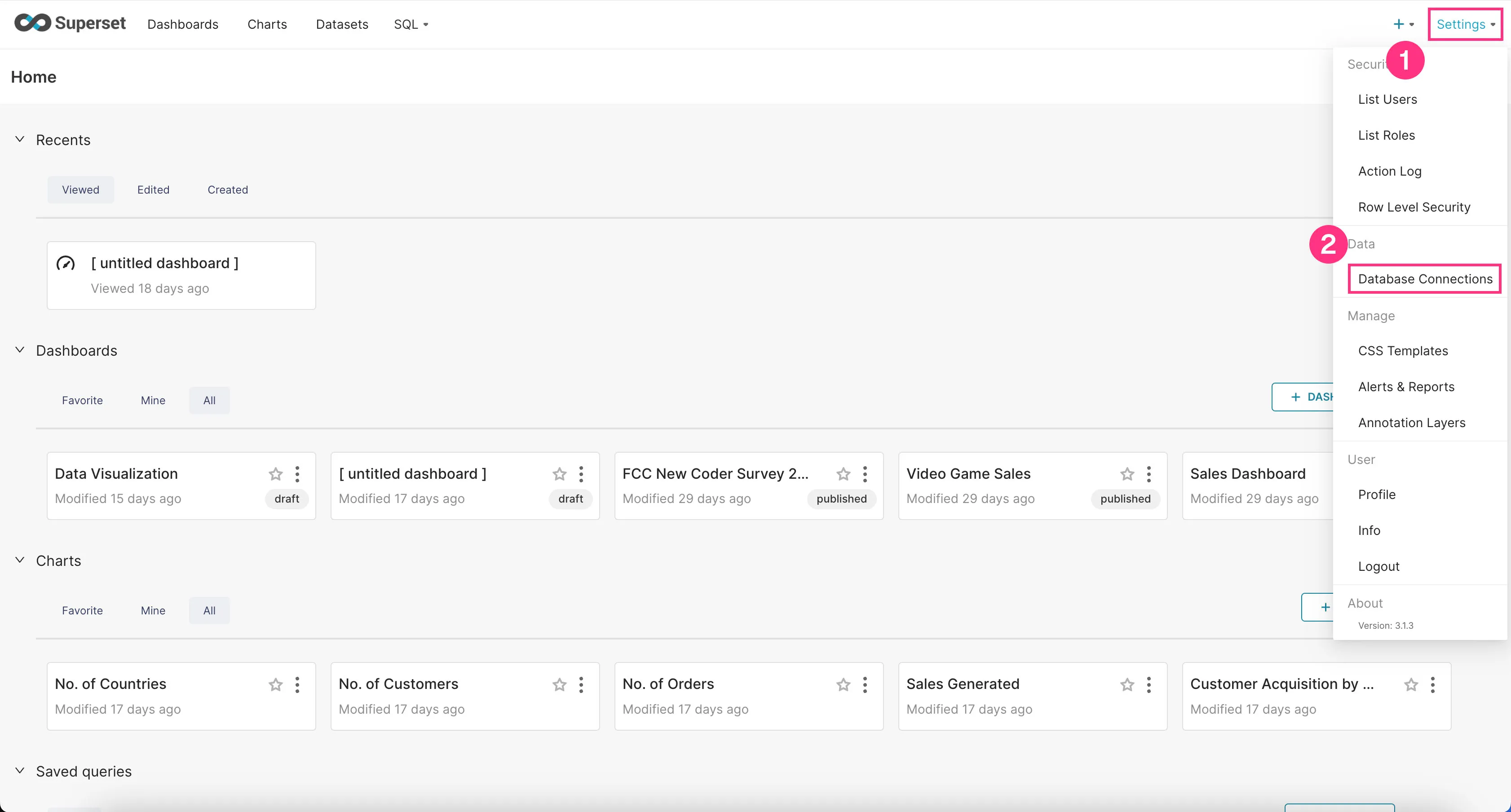
1. Go to the “Settings” dropdown at the top right corner and click “Database Connections”.

2. Click on the “+Database” button at the top right corner.

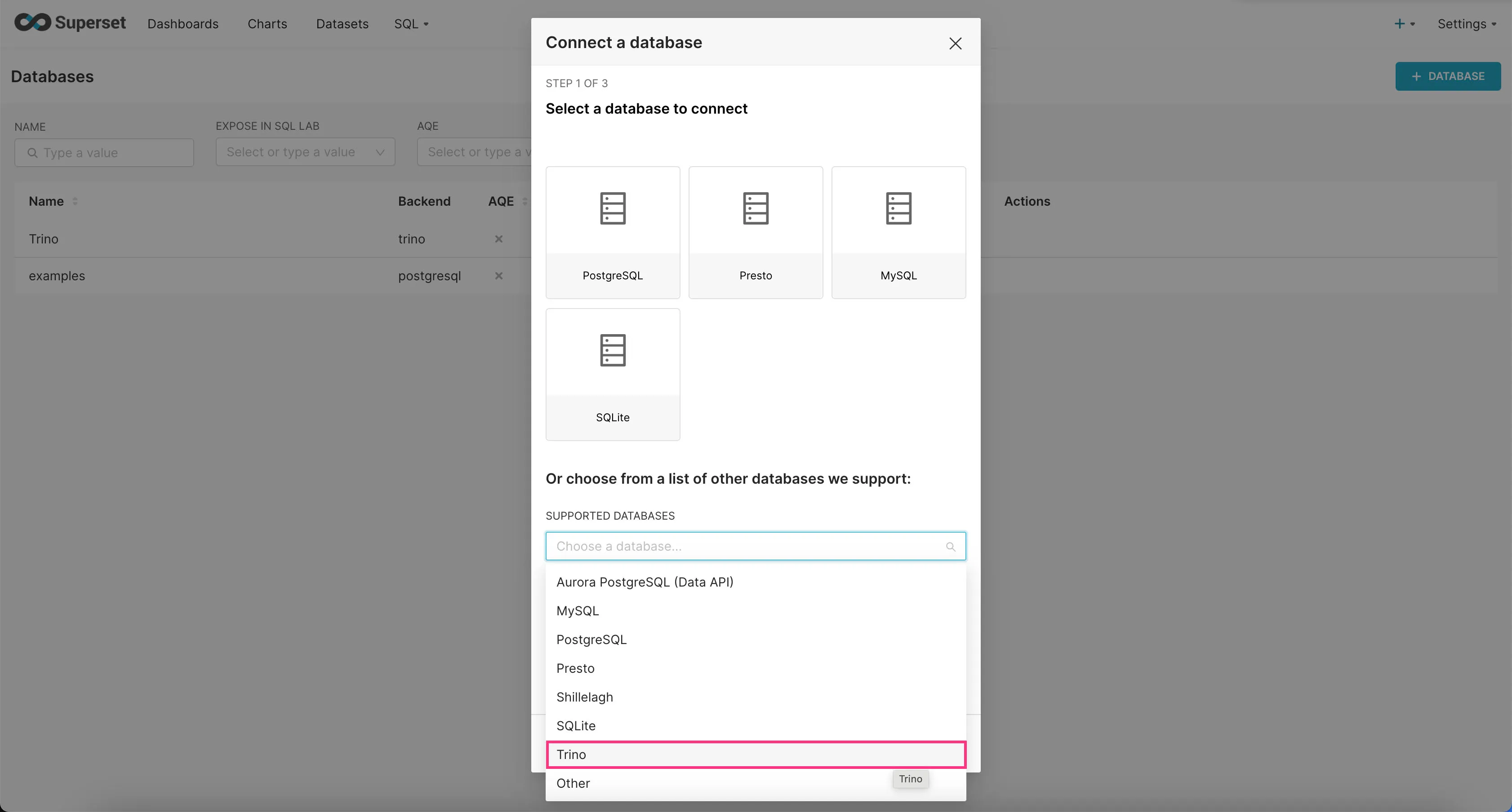
3. Find “Trino” option in the “SUPPORTED DATABASES” select field near the bottom.

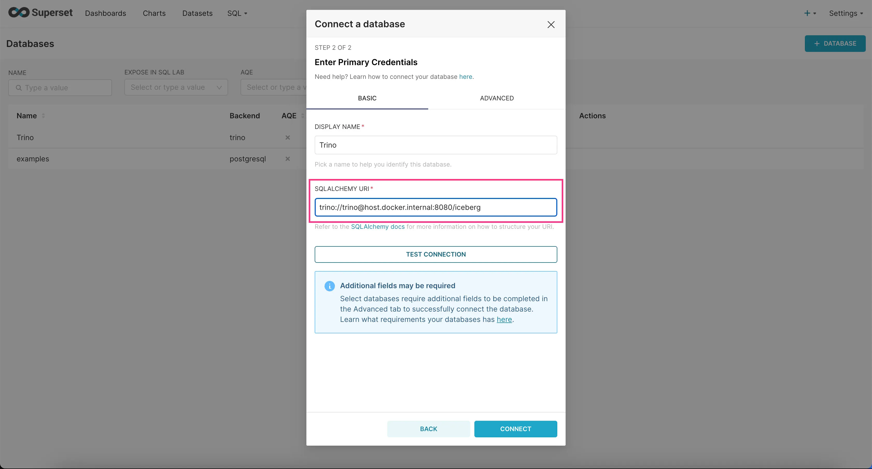
4. In the “SQLALCHEMY URI” field, enter trino://trino@host.docker.internal:8080/iceberg and then click “Connect”.

Trino should now be connected to Superset.

Add an Example Dashboard

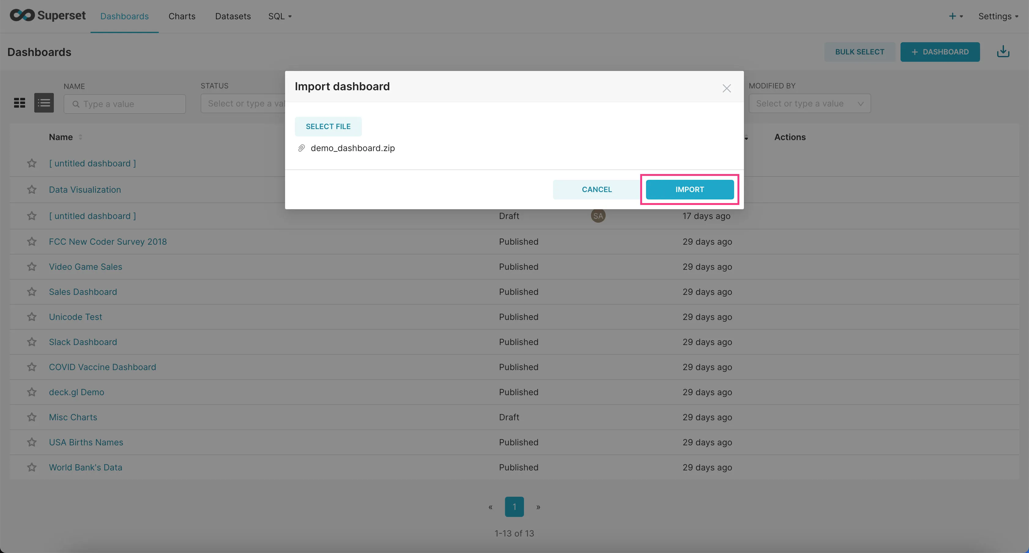
Now that we’ve connected Superset to Trino, let’s add an example dashboard we created for you.

1. First download the example dashboard here.
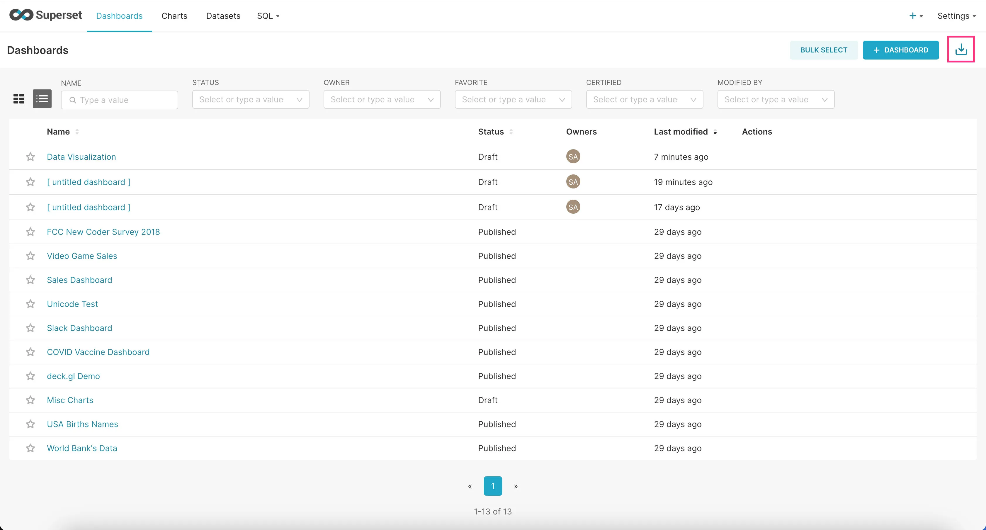
2. Go to the “Dashboards” tab and click on the Import Dashboard icon at the top-right corner.

3. Upload the downloaded zip file and click “Import”.

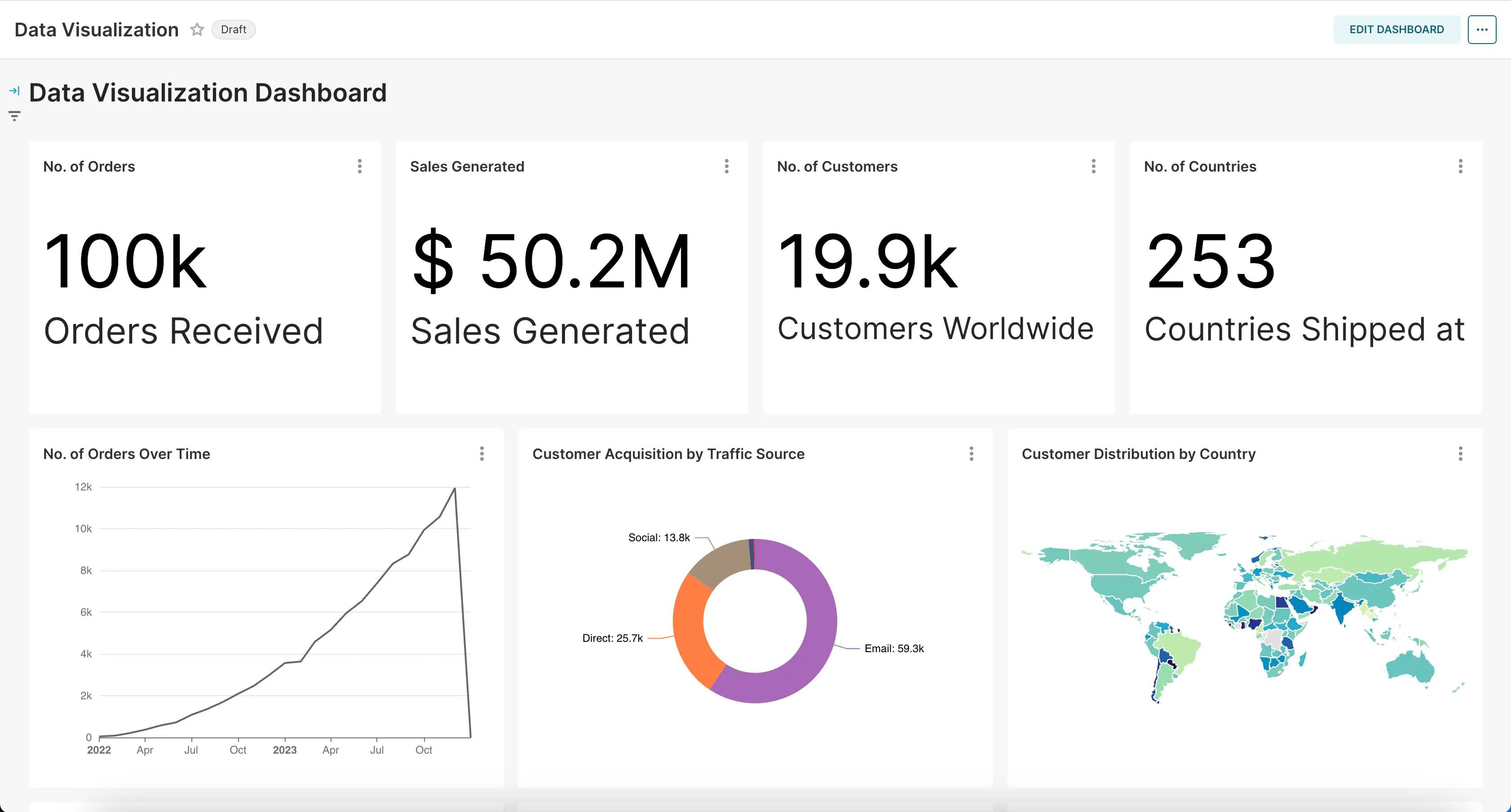
4. Find the example dashboard you just added in the list of dashboards and click on it to view it.

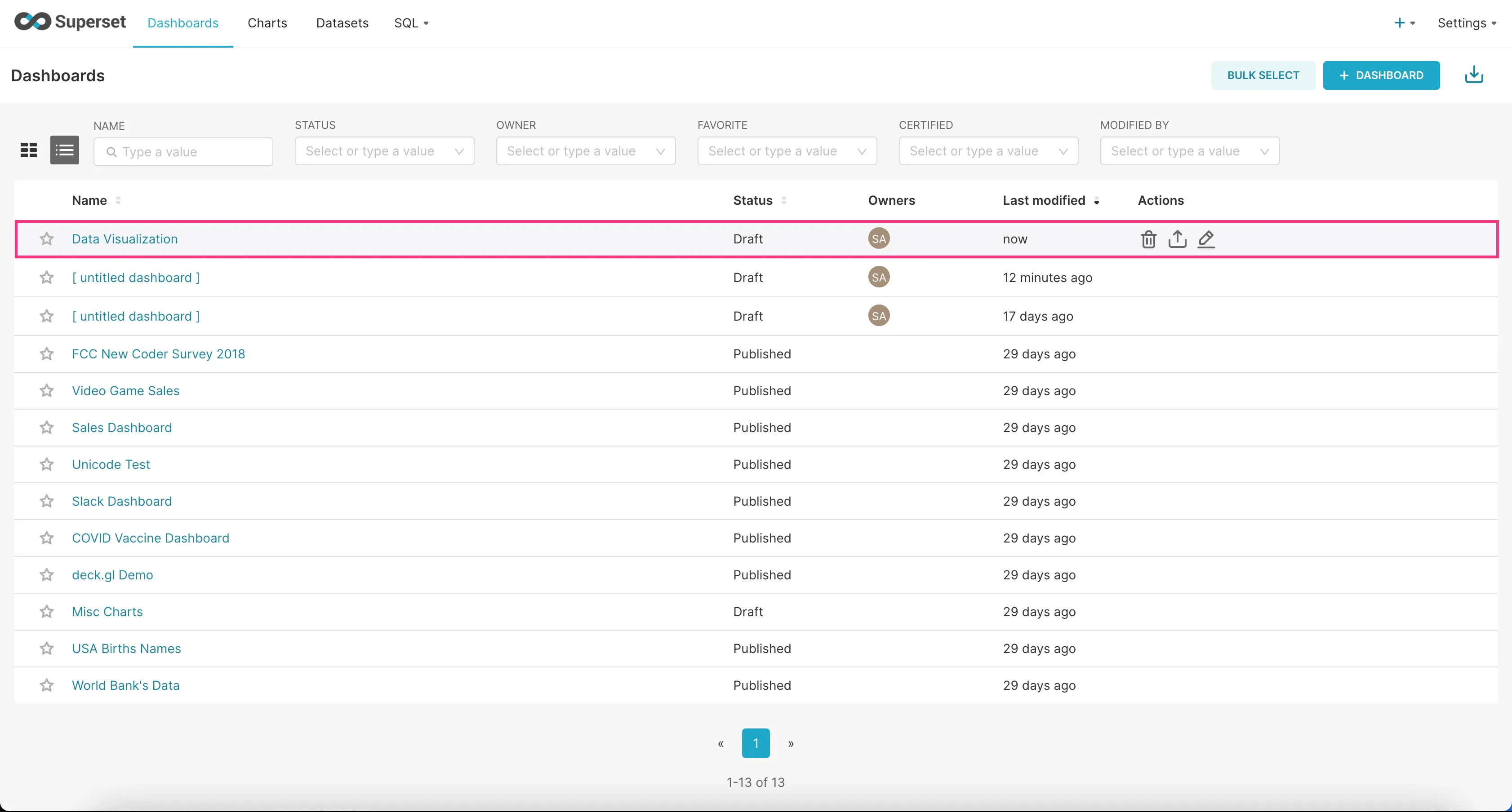
That’s it! You should now see a bunch of charts we created for you based on the example dataset.

Next Steps

Great! You should now have a better idea as to how this project setup can be used to run your data pipeline.

If you’re interested in digging deeper into how we built the example project step-by-step, check out the in-depth BI Stack Example Tutorial.